LLMs in JAX from scratch - Part 1
Build and pretrain a small language model in pure JAX.
In this series of blog posts, I will build and train LLMs from scratch using JAX. By “from scratch,” I mean using only pure JAX (JAX arrays, pytrees, etc.), without using any other framework (e.g., Flax). I will create a tiny neural network library that implements all the components needed to train LLMs.
The code for this series is available on GitHub.
I designed this series to reflect how I like to learn. Read more about my approach here.
Excellent resources
The mathematical explanations draw mainly on the following resources:
-
Formal Algorithms for Transformers: arXiv
-
Speech and Language Processing: Online textbook
-
Mathematical Foundations of Modern AI Systems: Lecture 1 or full course
Overall
My end goal is to pretrain a large language model (LLM). This entails training a neural network with a large number of parameters to predict the next word given the previous words using a very large corpus of text as training data.
Consider a sequence of words from this corpus,
| Input context | Target word |
|---|---|
I train the model by minimizing the cross-entropy loss, equivalently the average negative log-likelihood:
This loss encourages the model to assign a higher probability to the correct next word for each context.
Tokenization
Tokenization is a preprocessing step for training LLMs. It consists of segmenting raw text into tokens and assigning each token an integer ID. Tokens can represent whole words (e.g., dog, cat), parts of words (e.g., ing, ed, tion, ally), or characters (e.g., a, b, 😃). From this point on, the units of prediction are tokens rather than words.
There are different tokenization methods. Throughout this series, I use byte-level byte pair encoding (BPE). This process has two stages:
1. Training the tokenizer. I start by splitting the raw text into smaller pieces, such as words with their leading spaces. For example, "I have a new dog 😃" can be split into ["I", " have", " a", " new", " dog", " 😃"]. I then represent each piece as a sequence of bytes, which are numerical units used to store text. For example, "dog" becomes [100, 111, 103] in UTF-8, corresponding to d, o, and g. A character such as 😃 takes several bytes.
text = "dog"
print(list(text.encode("utf-8")))

text = "😃"
print(list(text.encode("utf-8")))
Output:
[100, 111, 103]
[240, 159, 152, 131]
A byte has 256 possible values. Initially, each byte is a token, so the word "dog" is represented by three token IDs: 100, 111, and 103. BPE then repeatedly merges the most frequent pair of adjacent tokens into a new token, without merging across the boundaries of the pieces defined above. Initially, these tokens are individual bytes; later, they can be tokens created by previous merges.
Training the tokenizer produces two things:
First, the vocabulary:
Each {97: b"a", 100: b"d", 103: b"g", 111: b"o"}. I initialize it with individual byte values and any special tokens. I choose the target vocabulary size
The following table shows selected entries from the vocabulary obtained by training BPE on the TinyStories dataset
| Token ID | Token, shown as readable text |
|---|---|
| 32 | ␠ |
| 97 | a |
| 256 | <|endoftext|> |
| 264 | ed |
| 300 | ing |
| 398 | ␠time |
| 430 | Once |
| 439 | ␠upon |
Here, ␠ represents a space. The entries are shown as readable text; internally, they store bytes.
Second, the merge rules, in the order they were learned. Each rule records which pair to merge and the ID of the new token. For example, these are three rules from the TinyStories tokenizer:
Rule 1:  b" "  + b"t"  → b" t"    (ID 257)
Rule 2:  b"h"  + b"e"  → b"he"    (ID 258)
Rule 7:  b" t" + b"he" → b" the"  (ID 263)
The last merge becomes possible after the earlier two have created b" t" and b"he".
2. Encoding the dataset. Once the vocabulary and merge rules are learned, I use them to encode the entire dataset for pretraining. Using the notation from the previous section, each text becomes a sequence
For example, using my TinyStories tokenizer:
"Once upon a time"
        ↓
["Once", " upon", " a", " time"]
        ↓
[430, 439, 259, 398]
These token IDs are what I feed into the model. To decode them, I look up their vocabulary entries, join the bytes, and convert them back to text.
Tokenizers trained on different data and with different vocabulary sizes can encode the same text differently. The examples below use a 10,000-entry vocabulary trained on TinyStories and a 50,257-entry vocabulary trained on OpenWebText (OWT) ␠software is one token in the OWT vocabulary and three in the TinyStories vocabulary.
| Input text | TinyStories tokenizer: tokens and IDs | OWT tokenizer: tokens and IDs |
|---|---|---|
␠software | ["␠soft", "w", "are"][1049, 119, 517] | ["␠software"][3476] |
␠algorithm | ["␠al", "g", "or", "ith", "m"][554, 103, 305, 326, 109] | ["␠algorithm"][11159] |
Custom networks with JAX
Throughout this series, I will use JAX to implement all the network layers from scratch. I register my layer classes as pytrees so JAX can access their parameter arrays when applying transformations such as jax.grad and jax.jit. Consider a linear layer, which has two trainable parameter arrays: a weight matrix
I start by implementing the math inside a class:
class Linear:
    def __init__(
        self, in_features: int, out_features: int, use_bias: bool = True, *, key: PRNGKeyArray
    ):
        self.in_features = in_features
        self.out_features = out_features
        self.use_bias = use_bias
        lim = 1 / math.sqrt(in_features)
        self.weight = uniform_init(key, (out_features, in_features), lim)
        self.bias = constant_init(shape=(out_features,), constant=0) if use_bias else None

    def __call__(self, x: Array) -> Array:
        x = x @ self.weight.T
        if self.use_bias:
            x = x + self.bias
        return x
I then use @register_pytree_with_keys_class to tell JAX how to flatten and unflatten a Linear instance. The documentation is provided here and here. In general, children contains parameter arrays and aux_data contains static metadata.
from jax.tree_util import GetAttrKey, register_pytree_with_keys_class

@register_pytree_with_keys_class
class Linear:
    ...
    def tree_flatten_with_keys(self):
        children = ((GetAttrKey("weight"), self.weight), (GetAttrKey("bias"), self.bias))
        aux_data = (self.in_features, self.out_features, self.use_bias)
        return (children, aux_data)

    @classmethod
    def tree_unflatten(cls, aux_data, children):
        obj = object.__new__(cls)
        obj.in_features, obj.out_features, obj.use_bias = aux_data
        obj.weight, obj.bias = children
        return obj
GetAttrKey("weight") labels a child with its attribute name. This helps with debugging and supports a custom jax_pprint helper that displays the layers and their parameter shapes. For example, once I have implemented TransformerLM, I can inspect it as follows:
model = TransformerLM(
    vocab_size=10000,
    context_length=128,
    num_layers=3,
    d_model=32,
    num_heads=4,
    d_ff=54,
    key=jax.random.key(0),
)
jax_pprint(model)
Output:
Model: TransformerLM
  token_embeddings: Embedding
    embeddings: shape=(10000, 32), dtype=float32
  blocks:
    [0]: TransformerBlock
      norm1: RMSNorm
        gain: shape=(32,), dtype=float32
      attn: MultiHeadSelfAttention
        w_query: Linear
          weight: shape=(32, 32), dtype=float32
          bias: None
        w_key: Linear
          weight: shape=(32, 32), dtype=float32
          bias: None
        w_value: Linear
          weight: shape=(32, 32), dtype=float32
          bias: None
        w_output: Linear
          weight: shape=(32, 32), dtype=float32
          bias: None
        rope: RoPE
      norm2: RMSNorm
        gain: shape=(32,), dtype=float32
      ff: FeedForward
        w1: Linear
          weight: shape=(54, 32), dtype=float32
          bias: None
        w2: Linear
          weight: shape=(32, 54), dtype=float32
          bias: None
        w3: Linear
          weight: shape=(54, 32), dtype=float32
          bias: None
    [1]: TransformerBlock
      norm1: RMSNorm
        gain: shape=(32,), dtype=float32
      attn: MultiHeadSelfAttention
        w_query: Linear
          weight: shape=(32, 32), dtype=float32
          bias: None
        w_key: Linear
          weight: shape=(32, 32), dtype=float32
          bias: None
        w_value: Linear
          weight: shape=(32, 32), dtype=float32
          bias: None
        w_output: Linear
          weight: shape=(32, 32), dtype=float32
          bias: None
        rope: RoPE
      norm2: RMSNorm
        gain: shape=(32,), dtype=float32
      ff: FeedForward
        w1: Linear
          weight: shape=(54, 32), dtype=float32
          bias: None
        w2: Linear
          weight: shape=(32, 54), dtype=float32
          bias: None
        w3: Linear
          weight: shape=(54, 32), dtype=float32
          bias: None
    [2]: TransformerBlock
      norm1: RMSNorm
        gain: shape=(32,), dtype=float32
      attn: MultiHeadSelfAttention
        w_query: Linear
          weight: shape=(32, 32), dtype=float32
          bias: None
        w_key: Linear
          weight: shape=(32, 32), dtype=float32
          bias: None
        w_value: Linear
          weight: shape=(32, 32), dtype=float32
          bias: None
        w_output: Linear
          weight: shape=(32, 32), dtype=float32
          bias: None
        rope: RoPE
      norm2: RMSNorm
        gain: shape=(32,), dtype=float32
      ff: FeedForward
        w1: Linear
          weight: shape=(54, 32), dtype=float32
          bias: None
        w2: Linear
          weight: shape=(32, 54), dtype=float32
          bias: None
        w3: Linear
          weight: shape=(54, 32), dtype=float32
          bias: None
  ln_final: RMSNorm
    gain: shape=(32,), dtype=float32
  lm_head: Linear
    weight: shape=(10000, 32), dtype=float32
    bias: None
The indentation shows how the layers are nested. Each array is displayed with its shape and data type; for example, the embedding table contains 10,000 vectors of size 32.
I will implement many custom layers, so writing these two methods in every class would be repetitive. Instead, I define a decorator that creates them and registers the class automatically. Each layer only needs to specify the attribute names for its children and aux_data:
def auto_pytree_with_keys(children: tuple[str, ...], aux_data: tuple[str, ...]):
    def decorator(cls):
        def tree_flatten_with_keys(obj):
            children_ = [(GetAttrKey(chld), getattr(obj, chld)) for chld in children]
            aux_data_ = tuple(getattr(obj, aux) for aux in aux_data)
            return children_, aux_data_

        def tree_unflatten(aux_data_, children_):
            obj = object.__new__(cls)
            for f, value in zip(children, children_, strict=True):
                setattr(obj, f, value)
            for f, value in zip(aux_data, aux_data_, strict=True):
                setattr(obj, f, value)
            return obj

        cls.tree_flatten_with_keys = tree_flatten_with_keys
        cls.tree_unflatten = tree_unflatten

        return register_pytree_with_keys_class(cls)

    return decorator
My Linear class then uses this decorator in place of @register_pytree_with_keys_class and the two explicit methods. Its initialization and forward computation stay the same:
@auto_pytree_with_keys(
    children=("weight", "bias"),
    aux_data=("in_features", "out_features", "use_bias"),
)
class Linear:
    ...  # Same __init__ and __call__ as above.
The transformer
I will build the transformer from four main components: token embeddings, normalization, multi-head attention, and a feed-forward network. The diagram shows how they fit together, with the transformer block repeated
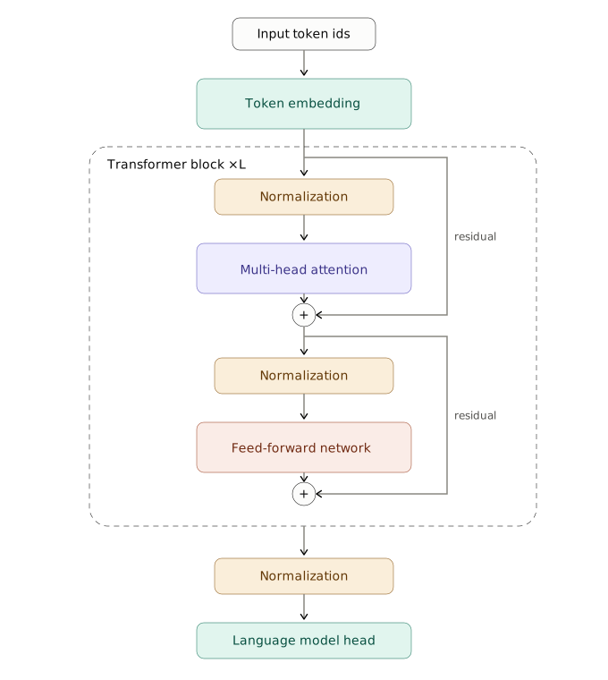
Token embedding
Token embedding assigns a trainable vector in
In JAX, I create a class that stores this matrix. Row
@auto_pytree_with_keys(
    children=("embeddings",),aux_data=("num_embeddings", "dim_embedding"))
class Embedding:
    def __init__(self, num_embeddings: int, dim_embedding: int, *, key: PRNGKeyArray) -> None:
        self.num_embeddings = num_embeddings
        self.dim_embedding = dim_embedding
        self.embeddings = normal_init(key, (num_embeddings, dim_embedding), std=0.02)

    def __call__(self, x: Int[ArrayLike, "..."]) -> Array:
        if not jnp.issubdtype(x.dtype, jnp.integer):
            raise TypeError(f"Inputs should be integers, got {x.dtype}")
        return self.embeddings.at[x].get(mode="fill", fill_value=jnp.nan)

    def decode(self, x: Array):
        return x @ self.embeddings.T
Positional information can be added alongside token embeddings to help the transformer represent token order. For example, “the dog bites the man” and “the man bites the dog” contain the same tokens but have different meanings. Token embeddings alone do not encode these differences in position.
There are different ways to represent position. One straightforward approach is to learn positional embeddings in the same way as token embeddings, using each token’s position in the sequence as the input instead of its ID.
I use rotary position embeddings (RoPE), which introduce positional information inside the multi-head attention layer. RoPE is explained later in this post.
Number of trainable parameters: the embedding layer has
Normalization
Normalization helps control the scale of neural network activations. I use root mean square normalization (RMSNorm). Given an activation vector
Here,
@auto_pytree_with_keys(children=("gain",),aux_data=("d_model", "eps"))
class RMSNorm:
    def __init__(self, d_model: int, eps: float = 1e-5) -> None:
        self.d_model = d_model
        self.eps = eps
        self.gain = jnp.ones((d_model,))

    def __call__(self, x: Array) -> Array:
        ms = jnp.mean(x**2, axis=-1, keepdims=True)
        x = x * jax.lax.rsqrt(ms + self.eps) * self.gain
        return x
Number of trainable parameters: the RMSNorm layer has
Multi-head attention
The multi-head attention (MHA) layer has four learnable projection matrices:
After embedding and normalization, the input to the MHA layer is
The next step is to compute attention scores. For each sequence in the batch, the score
Here,
A single head produces one attention weight for each token pair. However, tokens can be relevant to one another in several ways: one token might be the subject of another, or provide information about whether the subject is singular or plural. Multi-head attention allows the model to learn several attention patterns in parallel. With
To do this, I split the last dimension of
The following figure illustrates this:
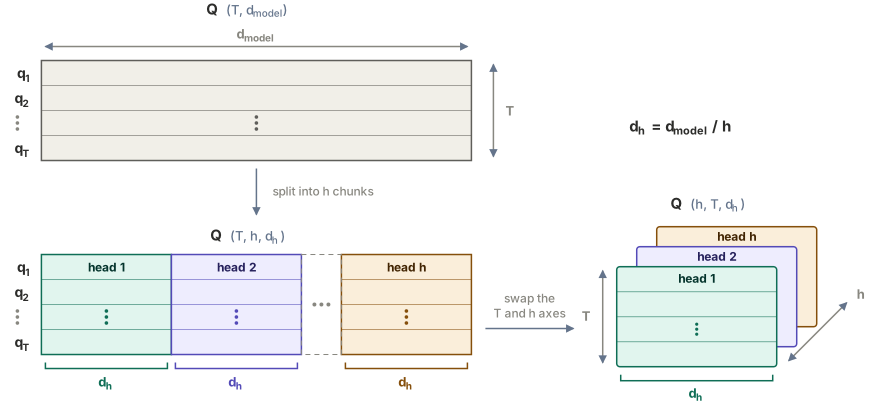
For each head
Here,
Finally, I concatenate the head outputs along the last axis and apply the output projection:
I first implement scaled dot-product attention in JAX. The following function returns the head output
def scaled_dot_product_attention(Q: Array, K: Array, V: Array, mask: None | Array = None):
    scores = (1 / math.sqrt(K.shape[-1])) * jnp.einsum("... a b, ... c b -> ... a c", Q, K)
    if mask is not None:
        scores = jnp.where(mask, scores, -jnp.inf)
    out = jnp.einsum("... a b, ... b c -> ... a c", jax.nn.softmax(scores, axis=-1), V)
    return out
I then use this function inside the multi-head attention layer. The RoPE step is explained in the next section.
@auto_pytree_with_keys(
    children=("w_query", "w_key", "w_value", "w_output", "rope"),
    aux_data=("d_model", "num_heads", "use_bias"),
)
class MultiHeadSelfAttention:
    def __init__(
        self,
        d_model: int,
        num_heads: int,
        use_bias: bool = False,
        rope: RoPE | None = None,
        *,
        key: PRNGKeyArray,
    ) -> None:
        assert d_model % num_heads == 0
        if rope is not None:
            assert rope.d_h == d_model // num_heads
        self.d_model = d_model
        self.num_heads = num_heads
        self.use_bias = use_bias
        self.rope = rope
        key1, key2, key3, key4 = jax.random.split(key, 4)
        self.w_query = Linear(
            in_features=d_model, out_features=d_model, use_bias=use_bias, key=key1
        )
        self.w_key = Linear(in_features=d_model, out_features=d_model, use_bias=use_bias, key=key2)
        self.w_value = Linear(
            in_features=d_model, out_features=d_model, use_bias=use_bias, key=key3
        )
        self.w_output = Linear(
            in_features=d_model, out_features=d_model, use_bias=use_bias, key=key4
        )

    def __call__(self, x: Array, token_positions: Array | None = None) -> Array:
        query = rearrange(self.w_query(x), "... seq (h d) -> ... h seq d ", h=self.num_heads)
        key = rearrange(self.w_key(x), "... seq (h d) -> ... h seq d ", h=self.num_heads)
        value = rearrange(self.w_value(x), "... seq (h d) -> ... h seq d ", h=self.num_heads)
        if self.rope:
            if token_positions is None:
                token_positions = jnp.arange(x.shape[-2])
            token_positions = token_positions[..., None, :]
            query = self.rope(query, token_positions)
            key = self.rope(key, token_positions)
        mask = jnp.tril(jnp.ones((x.shape[-2], x.shape[-2]), dtype=bool))
        out = scaled_dot_product_attention(Q=query, K=key, V=value, mask=mask)
        out = rearrange(out, "... h seq d -> ... seq (h d)")
        return self.w_output(out)
Number of trainable parameters: the bias-free MHA layer has
Rotary position embeddings (RoPE)
Consider two tokens: one at position
The goal is to make this score depend on the relative position of the tokens,
Here,
To obtain this score, I rotate the query and key as follows:
For any position
where
These rotations satisfy
I apply RoPE to queries and keys; the values stay unchanged.
For efficiency, I precompute and cache the cosine and sine values instead of constructing the full matrix
This is how I implement RoPE. I cache the cosine and sine values, then rotate each pair
from functools import cache
@cache
def rope_rotations(max_seq_len: int, d_h: int, theta: float):
    with jax.ensure_compile_time_eval():
        exponents = -jnp.arange(0, d_h, step=2) / d_h
        thetas = theta**exponents
        position = jnp.arange(max_seq_len)
        rotates = jnp.outer(position, thetas)
        rotates = jnp.repeat(rotates, 2, axis=-1)
        return jnp.cos(rotates), jnp.sin(rotates)  # of shape (max_seq_len,d_h)


@auto_pytree_with_keys(
    children=(),
    aux_data=("theta", "d_h", "max_seq_len"),
)
class RoPE:

    def __init__(self, theta: float, d_h: int, max_seq_len: int) -> None:
        self.theta = theta
        self.d_h = d_h
        self.max_seq_len = max_seq_len

    def __call__(self, x: Array, token_positions: Array) -> Array:
        coses, sines = rope_rotations(max_seq_len=self.max_seq_len, d_h=self.d_h, theta=self.theta)
        coses = coses[token_positions]
        sines = sines[token_positions]
        frst, scnd = jnp.unstack(rearrange(x, " ... (i j) -> ... i j", j=2), axis=-1)
        x_sins = rearrange(jnp.stack([-scnd, frst], axis=-1), "... i j -> ... (i j)")
        return x * coses + x_sins * sines
The RoPE class has no trainable parameters, so its children tuple is empty.
Feed-forward network
The feed-forward network applies the same transformation independently to each token. I use SwiGLU, which combines two projections through an elementwise product, then projects back to the model dimension:
Here,
I set
I implement this in JAX as follows:
def find_d_ff_(d_model: int, multiple_of: int = 64) -> int:
    d_ff = 8 * d_model / 3
    return multiple_of * round(d_ff / multiple_of)

@auto_pytree_with_keys(
    children=("w1", "w2", "w3"),
    aux_data=("d_model", "d_ff", "act_fun"),
)
class FeedForward:

    def __init__(
        self,
        d_model: int,
        d_ff: int | None = None,
        act_fun: Callable = jax.nn.silu,
        *,
        key: PRNGKeyArray,
    ) -> None:
        self.d_model = d_model
        self.act_fun = act_fun
        if d_ff is None:
            d_ff = find_d_ff_(d_model=d_model)
        self.d_ff = d_ff
        key1, key2, key3 = jax.random.split(key, 3)
        self.w1 = Linear(in_features=d_model, out_features=d_ff, use_bias=False, key=key1)
        self.w2 = Linear(in_features=d_ff, out_features=d_model, use_bias=False, key=key2)
        self.w3 = Linear(in_features=d_model, out_features=d_ff, use_bias=False, key=key3)

    def __call__(self, x: Array) -> Array:
        return self.w2(self.act_fun(self.w1(x)) * self.w3(x))
Number of trainable parameters: the feed-forward network has
Transformer block
I now assemble the normalization, multi-head attention, and feed-forward layers into a transformer block:
@auto_pytree_with_keys(
    children=("norm1", "attn", "norm2", "ff"),
    aux_data=(),
)
class TransformerBlock:
    def __init__(
        self,
        d_model: int,
        num_heads: int,
        d_ff: int | None = None,
        *,
        use_bias: bool = False,
        act_fun: Callable = jax.nn.silu,
        eps: float = 1e-5,
        rope: RoPE | None = None,
        key: PRNGKeyArray,
    ) -> None:
        key1, key2 = jax.random.split(key)
        self.norm1 = RMSNorm(d_model=d_model, eps=eps)
        self.attn = MultiHeadSelfAttention(
            d_model=d_model, num_heads=num_heads, use_bias=use_bias, rope=rope, key=key1
        )

        self.norm2 = RMSNorm(d_model=d_model, eps=eps)
        self.ff = FeedForward(d_model=d_model, d_ff=d_ff, act_fun=act_fun, key=key2)

    def __call__(self, x: Array, token_positions: None | Array = None) -> Array:
        x = x + self.attn(x=self.norm1(x), token_positions=token_positions)
        x = x + self.ff(self.norm2(x))
        return x
Number of trainable parameters: one transformer block with bias-free projections has
Transformer language model
I stack lm_head then projects the final normalized activations to logits of shape
@auto_pytree_with_keys(
    children=("token_embeddings", "blocks", "ln_final", "lm_head"),
    aux_data=("context_length",),
)
class TransformerLM:
    def __init__(
        self,
        vocab_size: int,
        context_length: int,
        num_layers: int,
        d_model: int,
        num_heads: int,
        d_ff: int | None = None,
        *,
        rope_theta: float = 10000.0,
        use_bias: bool = False,
        act_fun: Callable = jax.nn.silu,
        eps: float = 1e-5,
        key: PRNGKeyArray,
    ) -> None:
        assert d_model % num_heads == 0
        keys = jax.random.split(key, num_layers + 2)
        self.context_length = context_length

        rope = RoPE(theta=rope_theta, d_h=d_model // num_heads, max_seq_len=context_length)
        self.token_embeddings = Embedding(vocab_size, d_model, key=keys[0])
        self.blocks = tuple(
            TransformerBlock(
                d_model=d_model,
                num_heads=num_heads,
                d_ff=d_ff,
                use_bias=use_bias,
                act_fun=act_fun,
                eps=eps,
                rope=rope,
                key=keys[i + 1],
            )
            for i in range(num_layers)
        )
        self.ln_final = RMSNorm(d_model=d_model, eps=eps)
        self.lm_head = Linear(d_model, vocab_size, use_bias=False, key=keys[-1])

    def __call__(self, token_ids: Array, token_positions: Array | None = None) -> Array:
        x = self.token_embeddings(token_ids)
        for block in self.blocks:
            x = block(x, token_positions)
        return self.lm_head(self.ln_final(x))
Number of trainable parameters: the final RMSNorm has lm_head has
The following table summarizes the trainable parameter counts:
| Component | Trainable parameters |
|---|---|
| Token embeddings | |
| One transformer block | |
| Final RMSNorm | |
| LM head | |
| Total ( |
Interactive parameter explorer
Change the dimensions below to see how the parameter counts change throughout the transformer. Select a layer to see its calculation.
Training
I now train the model to predict the next token. For each batch, x contains the input token IDs and y contains their next-token targets. Both have shape
Loss function
I use the cross-entropy loss introduced at the beginning of this post. log_softmax computes the log probabilities directly for numerical stability. I then select the log probability of each target token and average its negative value over the batch and sequence positions:
def cross_entropy_loss(logits: Array, targets: Array) -> Array:
    loss = -jnp.take_along_axis(
        jax.nn.log_softmax(x=logits, axis=-1), indices=targets[..., None], axis=-1
    ).mean()
    return loss
AdamW optimizer
I implement AdamW from scratch. Given the gradient
Here, AdamWState and use jax.tree.map to apply the updates across the model:
class AdamWState(NamedTuple):
    lr: float
    beta_1: float
    beta_2: float
    decay: float
    eps: float
    step: int
    m: Any
    v: Any

def init_adamw(model, lr, beta_1, beta_2, decay, eps):
    return AdamWState(
        lr=lr,
        beta_1=beta_1,
        beta_2=beta_2,
        decay=decay,
        eps=eps,
        step=1,
        m=jax.tree.map(jnp.zeros_like, model),
        v=jax.tree.map(jnp.zeros_like, model),
    )

def update_adamw(model, grad, state):
    t, lr, decay = state.step, state.lr, state.decay
    beta_1, beta_2 = state.beta_1, state.beta_2

    alpha = lr * (1 - beta_2**t) ** 0.5 / (1 - beta_1**t)

    m = jax.tree.map(lambda m, g: beta_1 * m + (1 - beta_1) * g, state.m, grad)
    v = jax.tree.map(lambda v, g: beta_2 * v + (1 - beta_2) * g * g, state.v, grad)

    model = jax.tree.map(
        lambda p, m_, v_: p - lr * decay * p - alpha * m_ / (jnp.sqrt(v_) + state.eps), model, m, v
    )
    state = state._replace(m=m, v=v, step=t + 1)
    return model, state
Lazy data loading
After training the tokenizer, I tokenized the full dataset and saved it in a NumPy .npy file. To load it, I open it with mmap_mode="r". Memory mapping makes the required portions available on demand without loading the entire dataset into RAM.
def data_loading(data: Any, batch_size: int, context_length: int, rng):
    """
    Lazy loading of data
    """
    starts = rng.integers(0, len(data) - context_length, size=batch_size)
    idx = starts[:, None] + np.arange(context_length + 1)
    window = np.asarray(data[idx], dtype=np.int32)
    return jnp.asarray(window[:, :-1]), jnp.asarray(window[:, 1:])
window has shape
Training step
In the training script, I define the following functions inside train(args), after initializing the model and optimizer. loss_fn runs the model and computes the loss:
@jax.jit
def loss_fn(model, x, y):
    y_hat = model(token_ids=x)
    return cross_entropy_loss(logits=y_hat, targets=y)
train_step uses jax.value_and_grad to compute the loss and its gradients with respect to the model parameters. I measure the gradient norm, optionally clip the gradients, and apply the optimizer update:
@jax.jit(donate_argnums=(0, 1))
def train_step(model, optim_state, x, y):
    loss, grads = jax.value_and_grad(loss_fn)(model, x, y)
    grad_norm = global_norm(grads)
    if args.clip_grads > 0:
        grads = clip_grads(grads, args.clip_grads, eps=args.optim_eps, norm=grad_norm)
    model, optim_state = optim_update(model=model, grad=grads, state=optim_state)
    return model, optim_state, (loss, grad_norm)
The function returns the updated model and optimizer state, along with the loss and gradient norm. The optimizer and full training script will be provided on GitHub.
Results of training
I used this implementation to pretrain a language model on TinyStories. I rented an RTX 4090 GPU from Vast.ai for these experiments. The configurations, training curves, and run files are available in this public W&B project.
Training setup
With my 10,000-token vocabulary, the TinyStories training dataset contains 529,022,087 tokens. I used a context length of
This gives approximately 64,000 steps for a batch size of 32 and 32,000 steps for a batch size of 64.
The initial model has four transformer blocks,
I trained with AdamW and a cosine learning-rate scheduler, with warmup over the first 10% of training steps. I used
In my initial experiments, I tried batch sizes of 32 and 64, along with different values of
The table below shows the average training time over seven experiments for each batch size.
| Batch size | Training steps | Training time (minutes) |
|---|---|---|
| 32 | 64,000 | |
| 64 | 32,000 |
The best model I found in these initial experiments used
Parameter tying
With the dimensions of the four-block model entered in the interactive tool above, the token embedding and the LM head each have 5.12 million parameters. Together, they account for about 45% of the model: almost half of its parameters map token IDs to vectors at the input and project the final representations back to vocabulary scores at the output. I wanted to see whether I could allocate some of these parameters to the transformer blocks instead.
That is why I tried parameter tying. The idea is to use the same trainable matrix for the token embedding and the LM head. I keep the embedding matrix
The decode method in the Embedding layer already provides this projection:
class Embedding:
    ...

    def decode(self, x: Array):
        return x @ self.embeddings.T
In TransformerLM, I remove the separate lm_head from __init__ and from the pytree’s children tuple. I then use decode after the final normalization:
def __call__(self, token_ids: Array, token_positions: Array | None = None) -> Array:
    x = self.token_embeddings(token_ids)
    for block in self.blocks:
        x = block(x, token_positions)
    return self.token_embeddings.decode(self.ln_final(x))
This frees up 5.12 million parameters from the separate LM head. One transformer block needs about 3.11 million parameters, so I tried adding one or two blocks while keeping the total parameter count close to my original model. I also tried keeping four blocks and increasing the feed-forward width from 1,344 to 2,048. I used the best training configuration from the initial experiments for all of these architecture comparisons.
| Architecture | Blocks | Feed-forward width | Parameters | Validation loss | Training time (minutes) |
|---|---|---|---|---|---|
| Untied, four blocks | 4 | 1,344 | 22,696,448 | 1.2846 | 38.13 |
| Tied, extra block | 5 | 1,344 | 20,690,432 | 1.2456 | 44.79 |
| Tied, two extra blocks | 6 | 1,344 | 23,804,416 | 1.2254 | 51.82 |
| Tied, wider FFN | 4 | 2,048 | 21,901,824 | 1.2508 | 41.90 |
Training curves
The training times in the table are taken from the validation curves at step 64,000.
The six-block model gives the lowest loss, 1.2254, with about 4.9% more parameters than the four-block model. The five-block model also improves the loss while using fewer parameters. The figure below shows validation loss for the four-block model at a learning rate of 0.004 and the tied six-block model. Hover to compare values, or use the slider to zoom.
{"animation":false,"aria":{"enabled":true,"description":"Validation cross-entropy loss at every 1,000 training steps for the four-block model at lr 0.004 and the six-block tied model. Lower is better."},"color":["#ee7733","#228833"],"tooltip":{"trigger":"axis","axisPointer":{"type":"line"}},"legend":{"top":0,"type":"scroll","data":["Untied (4 blocks)","Tied (6 blocks)"]},"grid":{"top":55,"left":70,"right":20,"bottom":100},"xAxis":{"type":"value","name":"Training step","nameLocation":"middle","nameGap":30,"min":0,"max":64000},"yAxis":{"type":"value","name":"Validation loss ↓","min":1.2,"max":2.55,"nameGap":22},"dataZoom":[{"type":"inside","xAxisIndex":0,"filterMode":"none"},{"type":"slider","xAxisIndex":0,"bottom":15,"height":22,"start":0,"end":100,"filterMode":"none"}],"series":[{"name":"Untied (4 blocks)","type":"line","showSymbol":false,"smooth":false,"lineStyle":{"width":2.5},"data":[[1000,2.4250834780785815],[2000,2.0891570211427886],[3000,1.9693506303905126],[4000,1.8780701590201245],[5000,1.8137693908720651],[6000,1.7609346924413034],[7000,1.7092310658241494],[8000,1.663781369789171],[9000,1.632567119369909],[10000,1.6050350757666507],[11000,1.5870094259103977],[12000,1.5707291417105893],[13000,1.5570548334930523],[14000,1.5410904932319118],[15000,1.5330866113140873],[16000,1.5214471280546238],[17000,1.515108783540968],[18000,1.5054013685912793],[19000,1.4973246773179205],[20000,1.4889151967537135],[21000,1.483973238350503],[22000,1.4771087573370867],[23000,1.4678332385002395],[24000,1.4633699688548156],[25000,1.4580183876377575],[26000,1.4518082549712505],[27000,1.44630600143747],[28000,1.4403444313009104],[29000,1.4346595928665549],[30000,1.4284811856133206],[31000,1.4239942388895543],[32000,1.4173975053905128],[33000,1.4127389232450887],[34000,1.4062079802048395],[35000,1.4018458762577863],[36000,1.3950483087266412],[37000,1.3904717072951605],[38000,1.3834845359666985],[39000,1.3785184325586968],[40000,1.3738981267968375],[41000,1.3672602157702445],[42000,1.3627289096190704],[43000,1.3561585671717777],[44000,1.3513771075407284],[45000,1.3468025649856252],[46000,1.3412612863859608],[47000,1.3354834241734548],[48000,1.330693729036895],[49000,1.3257535487541927],[50000,1.3212467619489698],[51000,1.3168609809235745],[52000,1.3126390677407762],[53000,1.3088186354516052],[54000,1.304765550131768],[55000,1.3012891373682318],[56000,1.2986351521322472],[57000,1.2952985557918064],[58000,1.2931933546957355],[59000,1.2908022505390513],[60000,1.2892370365656445],[61000,1.2875046792644944],[62000,1.2863395424053665],[63000,1.2852909192321513],[64000,1.2846107413452323]]},{"name":"Tied (6 blocks)","type":"line","showSymbol":false,"smooth":false,"lineStyle":{"width":2.5},"data":[[1000,2.4226641111643508],[2000,2.049948340919981],[3000,1.9328896142788692],[4000,1.845732885122185],[5000,1.7732482705438428],[6000,1.7167474619669383],[7000,1.6611576126018208],[8000,1.613364540908002],[9000,1.5829650440225205],[10000,1.5546945188967418],[11000,1.5348192493711068],[12000,1.5198673147759942],[13000,1.5032641613260662],[14000,1.4887190419861045],[15000,1.4794805829240536],[16000,1.4664116779468137],[17000,1.459379960020364],[18000,1.450091619998802],[19000,1.4426406399736464],[20000,1.434276454689746],[21000,1.4281028202862962],[22000,1.420619178994969],[23000,1.412178253773359],[24000,1.4072463089961667],[25000,1.4010883969214183],[26000,1.3958078469393866],[27000,1.3895867647939626],[28000,1.3833999348646382],[29000,1.3769762405666028],[30000,1.37184093495448],[31000,1.3660227374820317],[32000,1.3605167405366554],[33000,1.3561462139135123],[34000,1.3494176187410158],[35000,1.3449046553066604],[36000,1.3377500598945855],[37000,1.332809037344274],[38000,1.3262292427827025],[39000,1.3209099484906563],[40000,1.3163778000718735],[41000,1.3096658630809774],[42000,1.3041350660337805],[43000,1.2985672092117873],[44000,1.2934625995747484],[45000,1.288262532942022],[46000,1.2827176045160518],[47000,1.2769682858169622],[48000,1.2719348010002396],[49000,1.2677104545999043],[50000,1.262396307498802],[51000,1.2581722418543364],[52000,1.2537625029947292],[53000,1.249929530276713],[54000,1.2457308262458073],[55000,1.2425513596070916],[56000,1.239336798484667],[57000,1.23649807588644],[58000,1.2342515610026354],[59000,1.231860644016531],[60000,1.230093472987542],[61000,1.2283520379132726],[62000,1.2271949493890753],[63000,1.2260609764314805],[64000,1.2253673222628174]]}]}
Sampling from the model
I now use the tied six-block model to generate text. Starting from a prompt, I predict the next token, append it to the context, and repeat. The sampling strategy determines how I choose each token from the model’s logits.
Sampling strategies
- Greedy: always choose the token with the highest logit.
def greedy_sampling(logits, **kwargs):
    return jnp.argmax(logits)
- Random: sample from the full vocabulary using
softmax(logits / temp). Temperature controls how concentrated the probabilities are. Lower values favor the most likely tokens; higher values allow more variety.
def random_sampling(logits, key, temp, **kwargs):
    return jax.random.categorical(key, logits / temp, axis=-1)
- Top-k: keep the
ktokens with the highest logits, then sample among them.
def top_k_sampling(logits, key, top_k, temp, **kwargs):
    k_logits, k_indices = jax.lax.top_k(logits, top_k)
    choice = random_sampling(k_logits, key, temp)
    return k_indices[choice]
- Top-p (nucleus): keep the most probable tokens whose cumulative probability reaches
p, then sample from that set.
def top_p_sampling(logits, key, top_p, temp, **kwargs):
    logits = logits / temp
    sorted_idx = jnp.argsort(-logits)
    sorted_logits = logits[sorted_idx]
    probs = jax.nn.softmax(sorted_logits)
    cum_probs = jnp.cumsum(probs)
    keep = (cum_probs - probs) < top_p
    masked = jnp.where(keep, sorted_logits, -jnp.inf)
    choice = jax.random.categorical(key, masked)
    return sorted_idx[choice]
Prompts and configurations
I use the configurations in the table below. Each configuration generates up to 256 new tokens per prompt.
| Strategy | Temperature | k | p | Configurations |
|---|---|---|---|---|
| Greedy | — | — | — | 1 |
| Random | 0.7, 0.9, 1.0 | — | — | 3 per seed |
| Top-k | 0.7, 0.9, 1.0 | 40, 50, 640 | — | 9 per seed |
| Top-p | 0.7, 0.9, 1.0 | — | 0.9, 0.95, 0.975 | 9 per seed |
I use the following prompts:
| Prompt | Text |
|---|---|
| 1 | Tom and Jane are friends. One day, Jane goes to Tom’s house. Tom has a big pot of soup. |
| 2 | Alice was so tired when she got back home so she went |
| 3 | Lily likes cats and dogs. She asked her mom for a dog and her mom said no, so instead she asked |
| 4 | Alice and Jack walked up the street and met a girl in a red dress. The girl said to them, |
| 5 | Once upon a time, in an ancient house, there lived a girl named Lily. |
| 6 | Once upon a time, there was a beautiful cat. |
Sampling results
I used an LLM judge to rate all 132 completions: 22 configurations, six shared prompts. Each criterion was scored out of 10:
- Grammar: correct sentences and word usage.
- Creativity: distinctive ideas, rather than repetition or random incoherence.
- Consistency: stable characters and events that agree with the prompt.
- Plot coherence: connected events and a supported ending.
The table shows the highest-scoring setting per method. Overall is the equally weighted average of the four criteria.
| Setting | Grammar | Creativity | Consistency | Plot coherence | Overall |
|---|---|---|---|---|---|
| Top-p, T=0.7, p=0.975 | 8.3 | 3.5 | 6.0 | 5.5 | 5.8 |
| Random, T=0.7 | 8.2 | 3.7 | 6.0 | 4.8 | 5.7 |
| Top-k, T=0.7, k=40/50/640 | 7.7 | 2.7 | 5.7 | 4.5 | 5.1 |
| Greedy | 8.8 | 2.2 | 4.2 | 3.8 | 4.8 |
Greedy has the highest grammar score (8.8) but the lowest creativity (2.2) among all 22 settings.
The five highest overall scores are listed in the table below. Four of the five configurations use top-p.
| Configuration | Grammar | Creativity | Consistency | Plot coherence | Overall |
|---|---|---|---|---|---|
| Top-p, T=0.7, p=0.975 | 8.33 | 3.50 | 6.00 | 5.50 | 5.83 |
| Top-p, T=0.9, p=0.9 | 8.33 | 3.67 | 5.67 | 5.33 | 5.75 |
| Random, T=0.7 | 8.17 | 3.67 | 6.00 | 4.83 | 5.67 |
| Top-p, T=0.7, p=0.95 | 8.67 | 2.67 | 6.50 | 4.67 | 5.62 |
| Top-p, T=0.9, p=0.95 | 8.33 | 4.17 | 5.33 | 4.67 | 5.62 |
Generated examples
Illustrative examples from prompt P4. Generated wording is unchanged; only the terminal <|endoftext|> marker is removed.
Prompt P4:
Alice and Jack walked up the street and met a girl in a red dress. The girl said to them,
Top-p, T=0.7, p=0.975
“I am very poor and I need some money to buy some food.” Alice and Jack were very kind, so they said, “We will help you. We will all buy food and you will be happy.” The girl was very happy and thanked Alice and Jack. They all went back to the park and started to eat the food. They were having a great time and the girl was very happy too. At the end of the day, the girl thanked Alice and Jack for their help and said, “Thank you for the food and for helping me. You are very kind.” Alice and Jack smiled and said, “We are happy to help. It made us feel good and strong!” The girl gave them a big hug and thanked them again. Alice and Jack waved goodbye, knowing that they had done something kind and compassion.
Greedy
“Hi, I’m Lucy. What’s your name?” Alice said, “I’m Alice. I’m Alice.” Lucy said, “Do you want to play with me?” Alice said, “Yes, let’s play!” Alice and Jack played together all day. They ran around the street and laughed. Alice was so happy to have a new friend. At the end of the day, Alice said goodbye to Jack and thanked him for playing with her. She said, “Bye, Jack. See you soon!” Alice and Jack waved goodbye and Alice went home. She was so happy to have made a new friend.
Top-k, T=0.9, k=50
“I wish your luck was to see my house. Can your house come with you?” Alice smiled and said, “Yes, of course! I can help”. She showed the little boy how to bring the items to her house. The old lady thanked Alice for her help and said, “Thank you for your help! I can’t wait to see your house.” Alice smiled proudly and said, “I’m so happy I’m ready to help”. The old lady replied, “Well, why don’t you come visit me again? You will always be welcome to your big house”. Alice thanked the old lady and went home with a big smile.
What is next
Next, I will focus on optimizing the code. We will focus on:
- How to profile JAX code
- How to optimize the network layers and training code.
- Add a KV cache to speed up text generation.
Enjoy Reading This Article?
Here are some more articles you might like to read next: